There are two ways to quickly change the formatting of a chart in excel so it is exactly the same as another chart. This is useful if you need to make lots of charts that all need to look the same, so you don’t have to repeat the same process over and over again.
Method 1: Chart Template
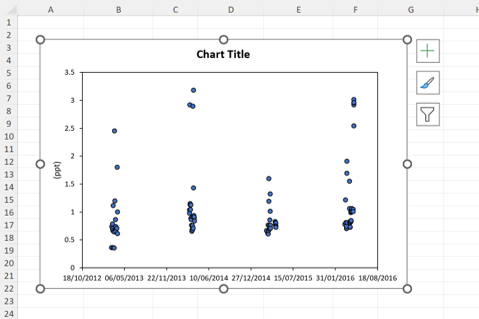
1. Use the keyboard shortcut Alt + F1 to make a chart.
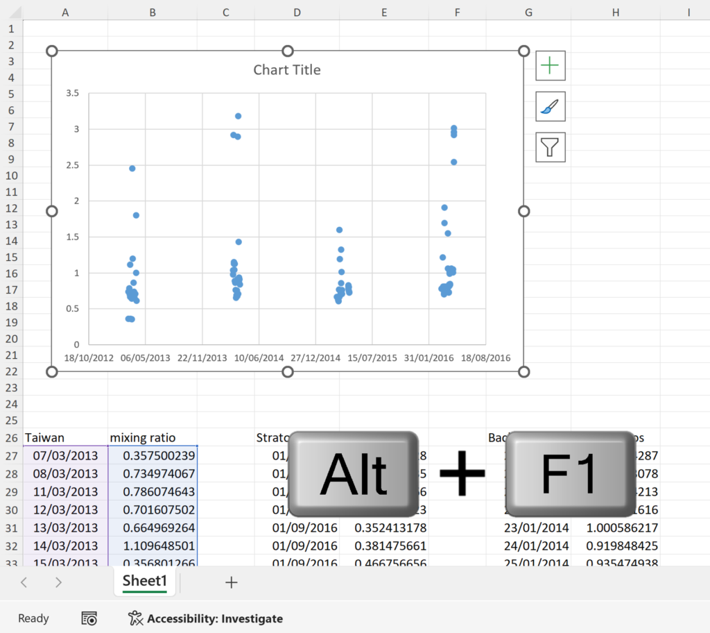
2. Format this chart exactly the way you want it.
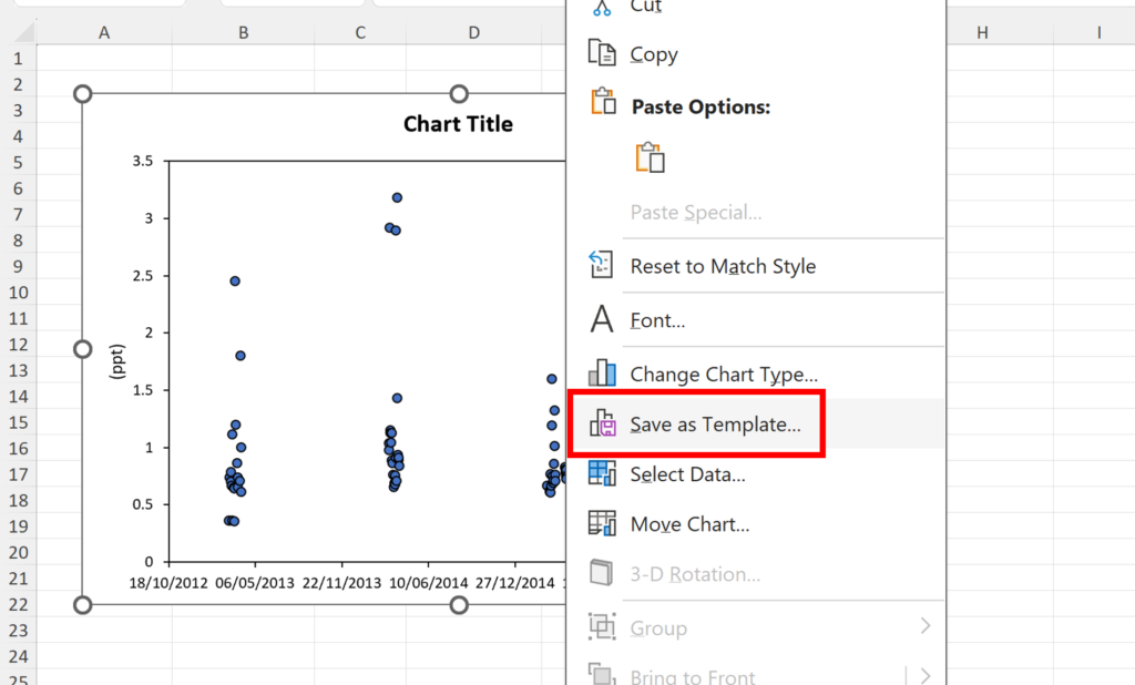
3. Right click on the chart and select Save as Template…
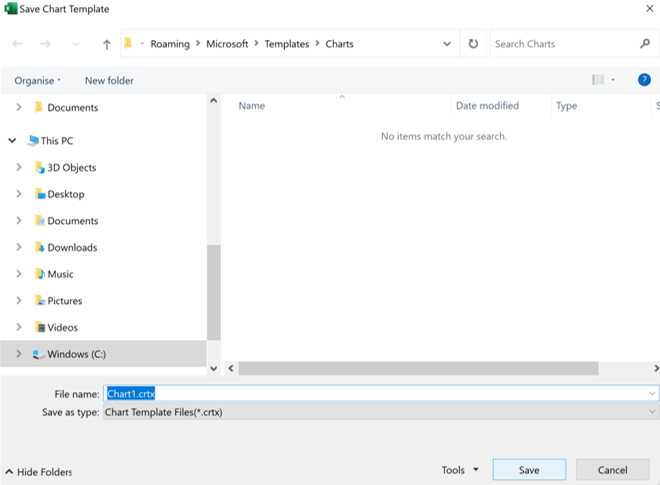
4. The default name is Chart1, you can change it to whatever you want, and then save the template.
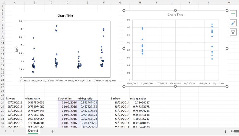
5. Make a new chart using different data.
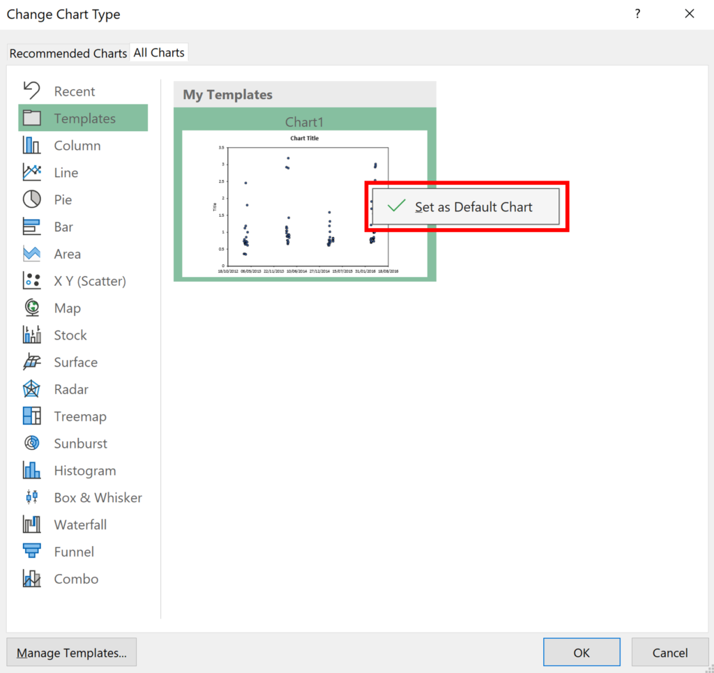
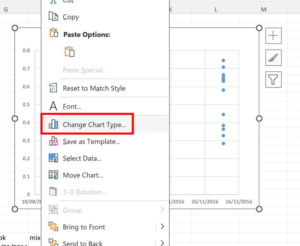
6. Right click on the new chart and select Change Chart Type…
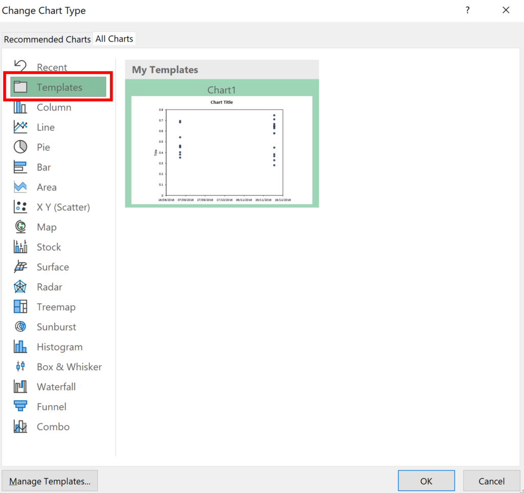
7. Go to Templates and select the chart template you just made.
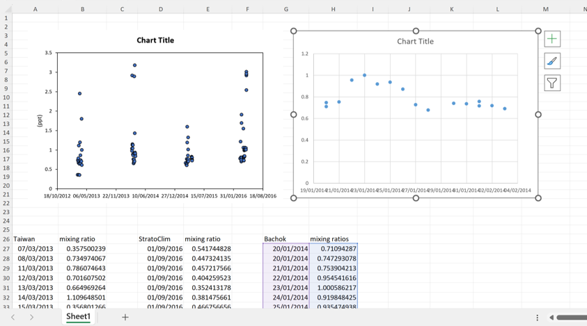
8. The formatting of the new chart will change to match the original.
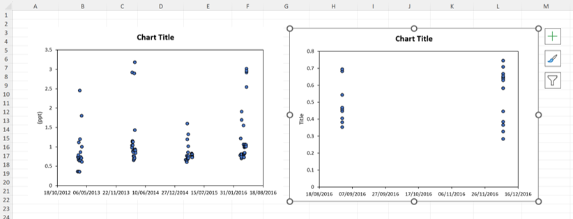
There are some limiations with this, for example if you set the axis maximum and minimum values in the original chart, that will be tranferred across to the new chart. So if you want the axes to adjust to the new data, you have to leave the axis maximum and minimum as automatic.
You can make multiple different templates and these will be available in all of your excel worksheets.
Method 2: Paste Special
1. Make a new chart using different data.
2. Select the original chart that has the formatting you want and copy the chart.
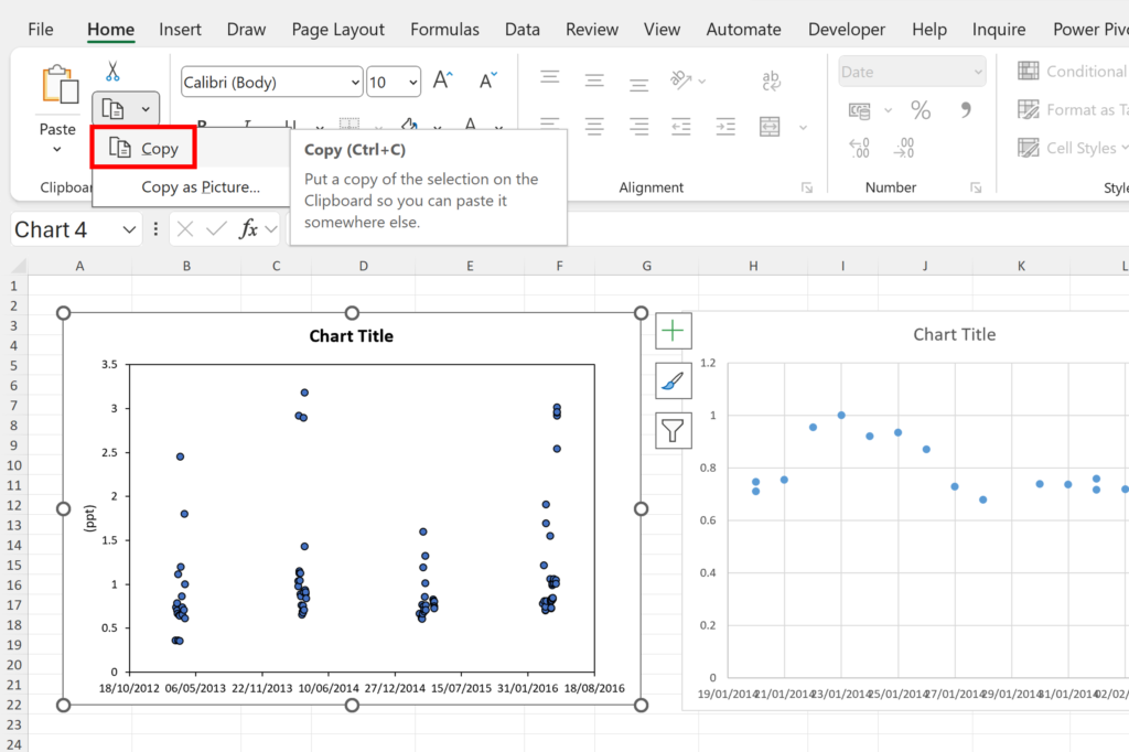
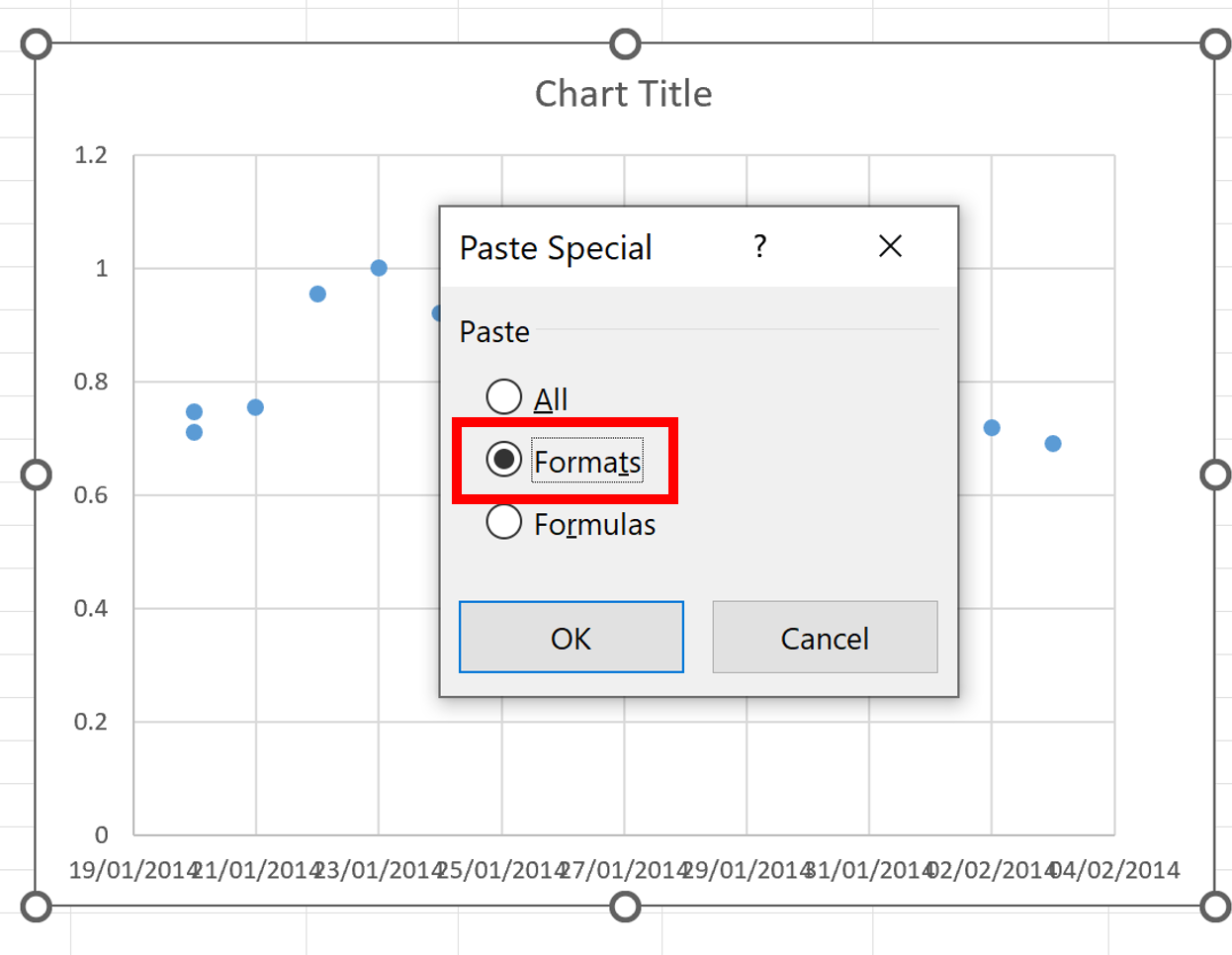
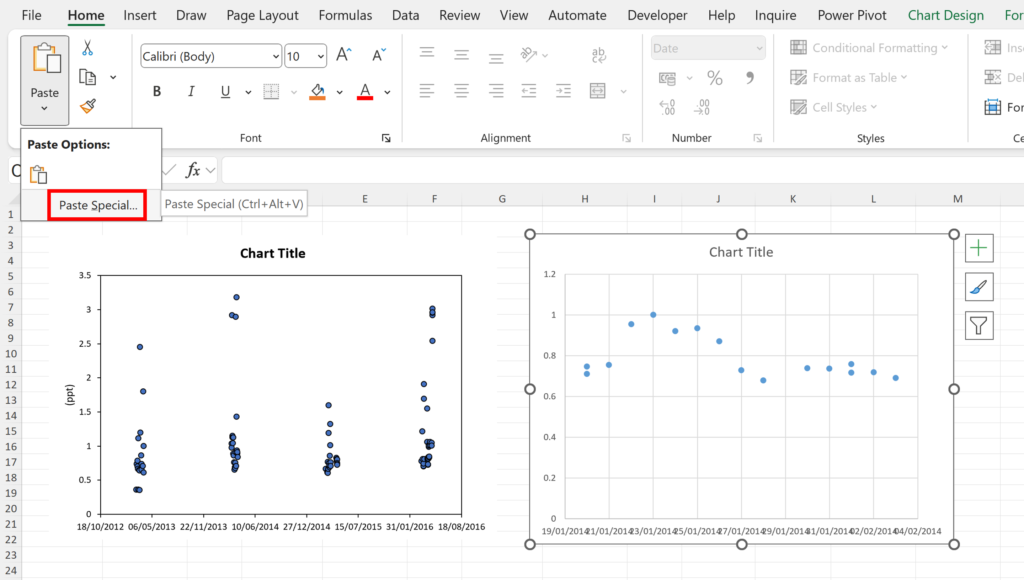
3. Next, select the new chart. Click Paste and then Paste Special.
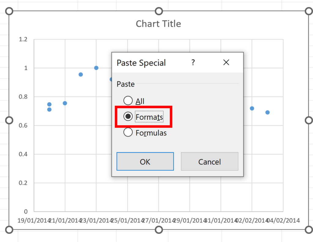
4. Paste the Formats.
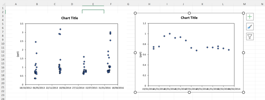
5. The formatting from the original chart has now been copied to the new chart. So the original chart and the new chart now have the same formatting.
Bonus Tip
You can set a chart as the default chart, so that will be the chart that is used when you make a chart using the keyboard shortcut Alt + F1.