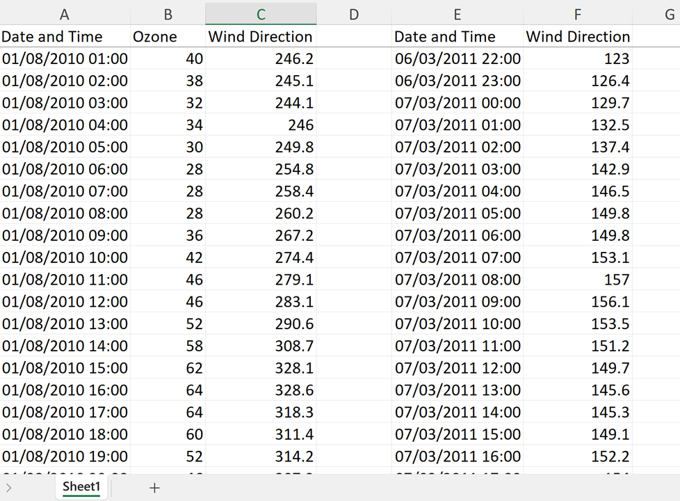
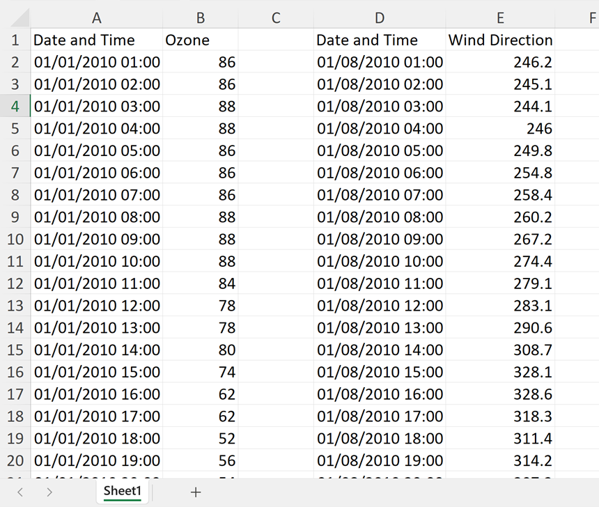
The data comes from the UK-AIR DEFRA website and is hourly atmospheric ozone concentrations and modelled wind direction at Weybourne Atmospheric Observatory in the UK 2010-2014. There are some gaps in the wind direction data so the tables don’t line up. In order to line up the wind directions with the ozone concentrations an INDEX MATCH formula is used.
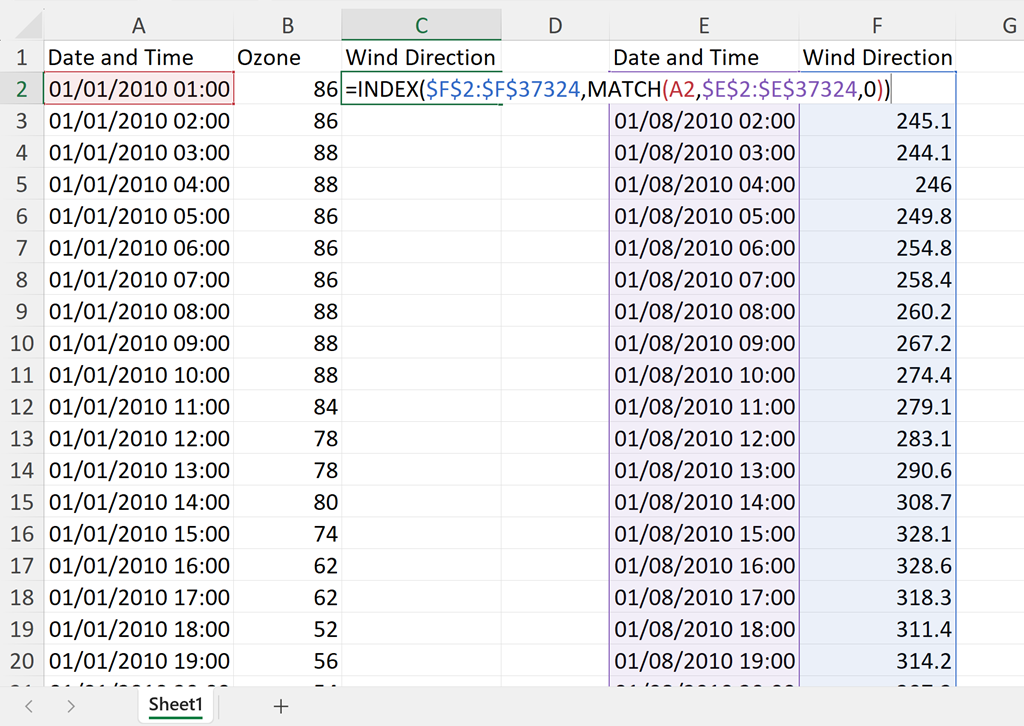
In a new column, put the following formula:
=INDEX($F$2:$F$37324,MATCH(A2,$E$2:$E$37324,0))
=INDEX(array, row_num)
The array is the column with the wind direction. Press F4 to insert the dollar signs to turn this into an absolute cell reference so it doesn’t change when the formula is filled down.
The row_num is the MATCH function
=MATCH(lookup_value, lookup_array, [match_type])
The lookup_value is the value we want to find, which is the date and time in the ozone table.
The lookup_array is the range we want to find the lookup_value in, which is the date and time in the wind direction table. Press F4 again to make this an absolute cell reference.
The match_type has to be zero for an Exact Match.
The MATCH function gives a number based on the position of the lookup_value in the lookup_array.
This then becomes the row_num in the INDEX function.
The INDEX function will find the wind direction for that date and time.