Summary
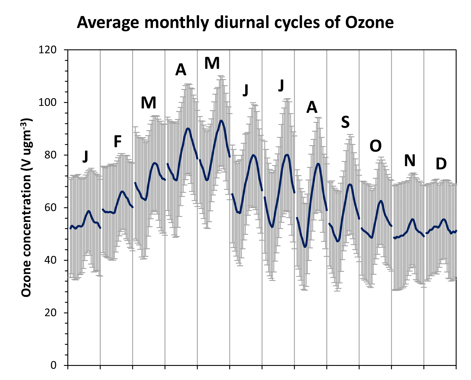
Use a pivot table to calculate the one sigma standard deviation of the variation in ozone concentrations during the whole of the measurement period and then insert error bars into the chart of one standard deviation.
Step by Step guide
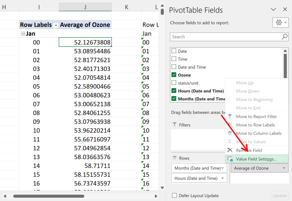
1. I’m using the Pivot Table and Chart that I made in a previous post. The data comes from the UK-AIR DEFRA website and is hourly atmospheric ozone concentrations at Weybourne Atmospheric Observatory in the UK 2010-2014.
2. In the Pivot Table Values field right click on Ozone and go to Value Field Settings
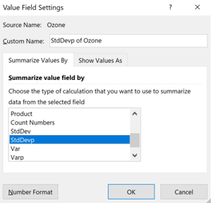
3. Change the Value to StdDevp, i.e. standard deviation of the population
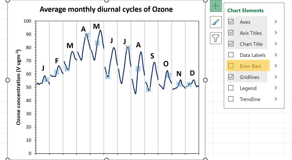
4. On the Chart, select the Series and then click on the green plus in the corner and add in Error Bars
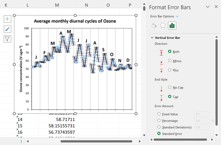
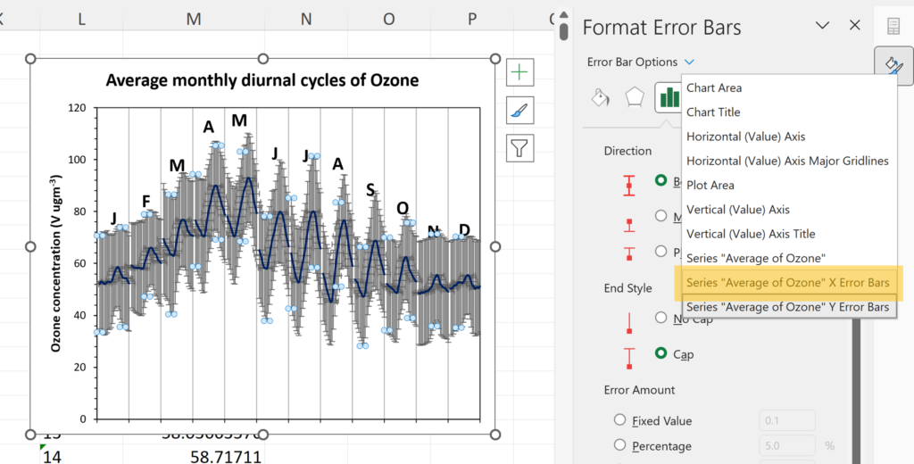
5. Double click on the error bars to open up the format bar
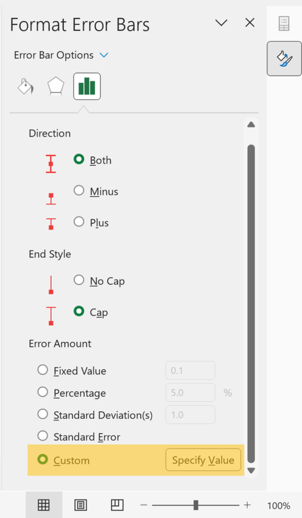
6. Change the Error Amount to Custom and click on Specify Value
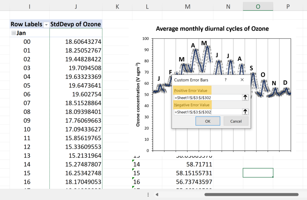
7. Select the whole of the standard deviation column for both the Positive and Negative values
8. Use the drop down list at the top of the format bar to select the X Error Bars and use Delete on the keyboard to remove them.
Final Result