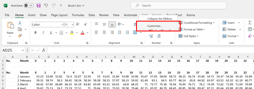
1. To do this you need the Developer tab. Right click on the Tabs at the top and then select Customize…
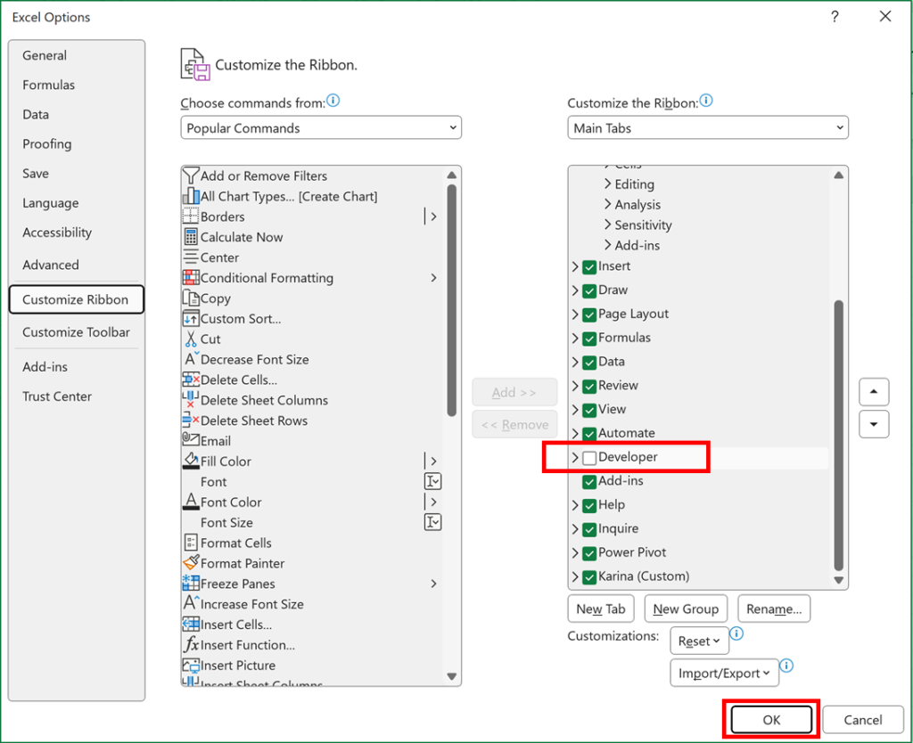
2. Tick the Developer box and select OK
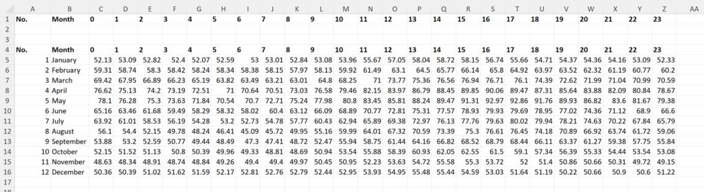
3. In this example there is a table with hours of the day along the top and months down the side. There is an extra copy of the headings just above the table.
The original data comes from the UK-AIR DEFRA website and is hourly atmospheric ozone concentrations at Weybourne Atmospheric Observatory in the UK 2010-2014.
4. In the first cell, put the number one. In the second cell put the following VLOOKUP formula.
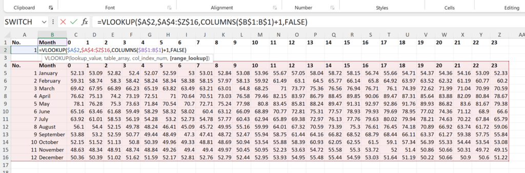
=VLOOKUP($A$2,$A$4:$Z$16,COLUMNS($B$1:B$1)+1,FALSE)
=VLOOKUP(lookup_value,table_array,col_index_num,[range_lookup])
The lookup_value is this number one you just typed in. Press F4 to put dollar signs around this cell reference so that it is an absolute cell reference and it doesn’t change when you drag the formula across.
The table_array is the whole of the table. Again press F4 to make it an absolute cell reference.
The col_index_num is the column number you want it to show you the results from. We use the COLUMNS function. The first cell reference has dollar signs in front of both the column letter and the row number and the second cell reference has a dollar sign in front of just the row number. So the range will expand as you drag the formula across and the number of columns will increase. You need to add one to this to account for the number column in the first column of the table.
The range_lookup needs to be FALSE for an exact match.
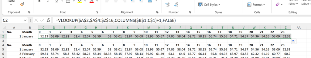
5. Drag the VLOOKUP formula across to fill the whole row.
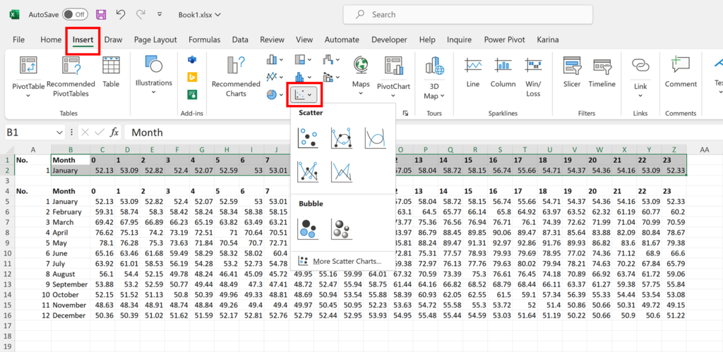
6. Select the top two rows and Insert a Scatter Chart.
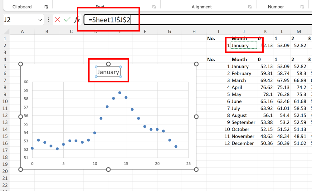
7. Select the Chart Title and click in the formular bar and then select the cell with the name of the month, to make the chart title dynamic.
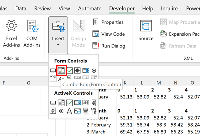
8. Insert a dropdown box by clicking on the Developer tab and then select Insert Form Controls and then Combo Box.
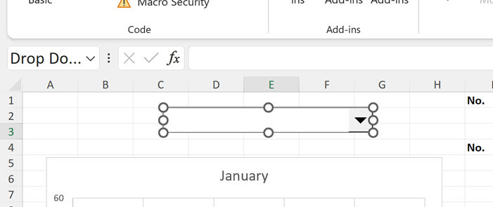
9. Click and drag to draw the dropdown box.
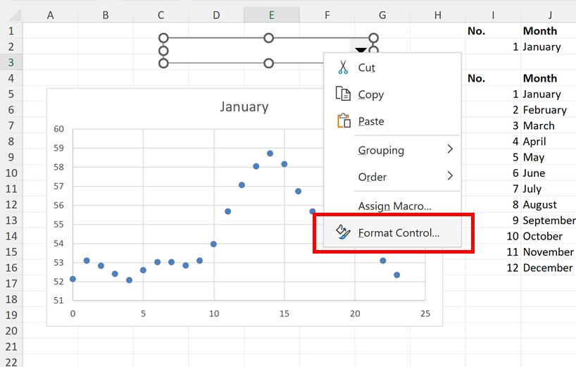
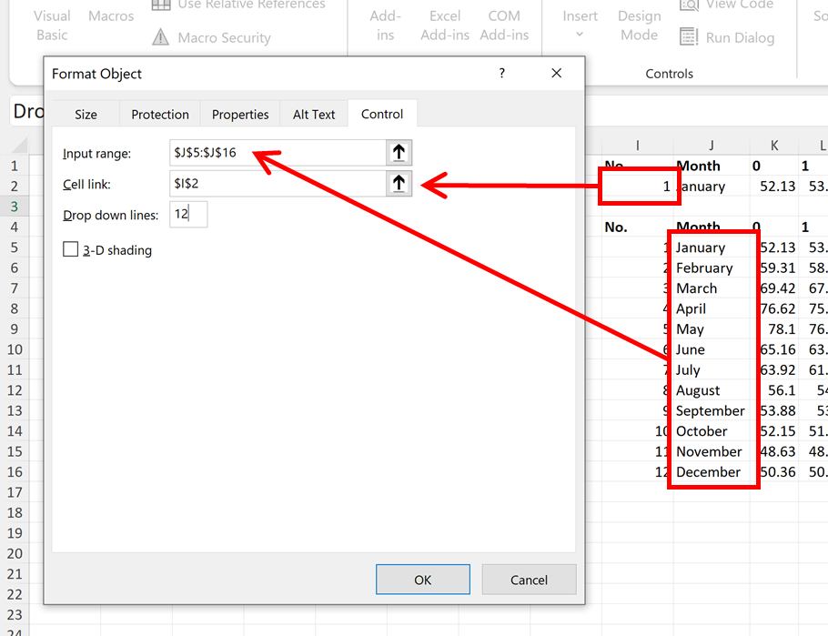
10. Right click the dropdown box and select Format Control.
11. The Input range is whatever you want to show up in the dropdown list. Select the column with the names of the months.
The Cell link is the cell that the dropdown box will change. In this example its cell I2, the cell we put the number one into in Step 4.
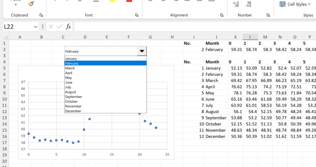
Change the Drop down lines from 8 to 12, as there are 12 months in the year and we want to see all of them when the dropdown box is selected.
12. When you press OK it will automatically change to the number in cell I2 to zero and mess up the formulas and the chart.
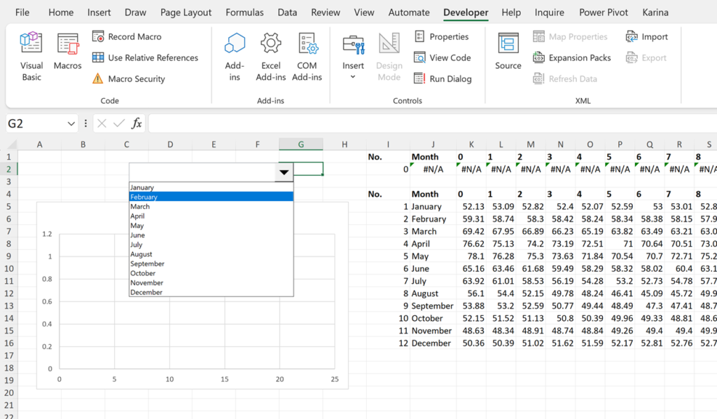
Click off the dropbox box to get out of Design mode. Then click the dropdown box again and now a dropdown list will appear with all of the months, and you can click on one to select it.
The number in cell I2 will change and this will make the results of all the VLOOKUP formulas change as they are all linked to that cell. As the chart is plotting the results of the VLOOKUP formulas this will also change the chart.
Now the chart is dynamic.
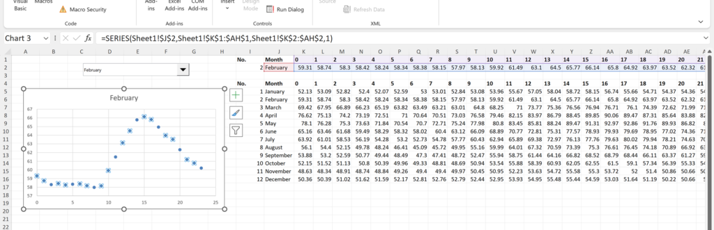
Final Result