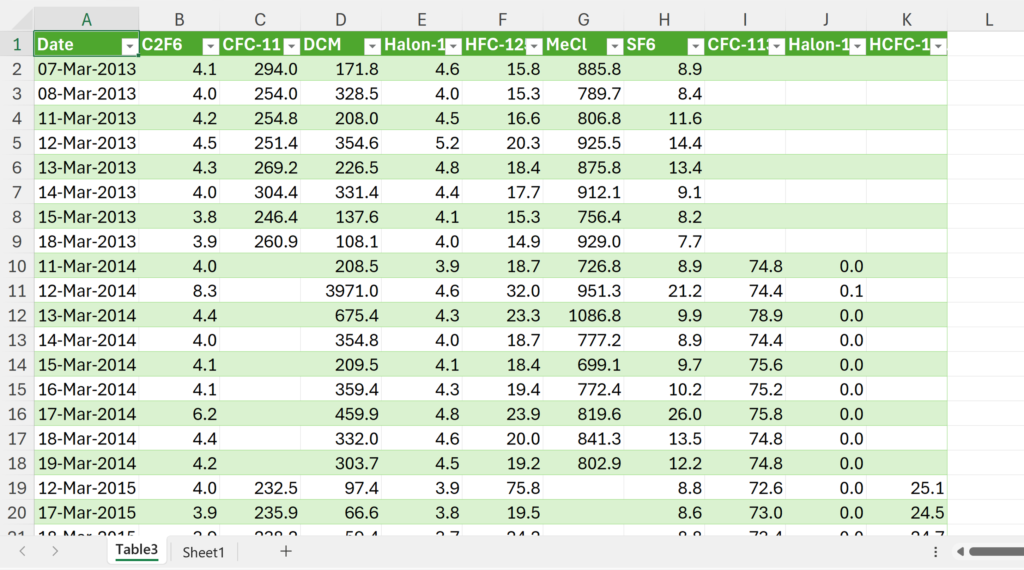
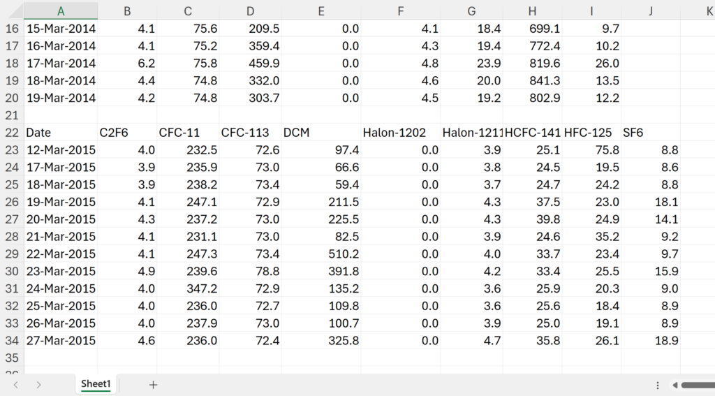
In this example, I have three tables, for each year: 2013, 2014 & 2015.
I want to combine these tables together but they don’t all have the same columns. So I will use Power Query to do this. In Power Query the columns will automatically line up so long as they have the same column headings.
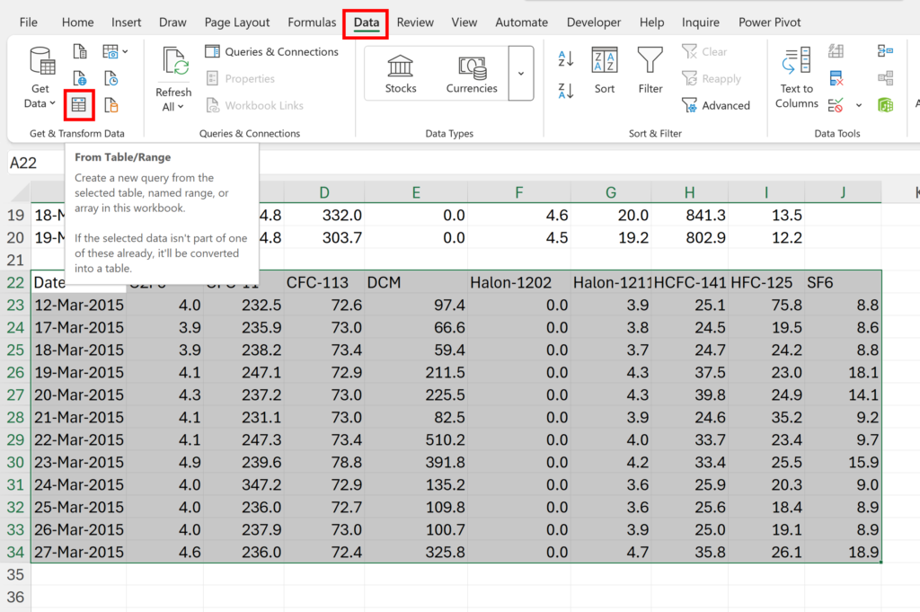
Firstly, for each of the tables, (I will be going backwards from the last table to the first table), select the whole table. On the Data Tab, in the Get & Transform Data section, click From Table/Range.
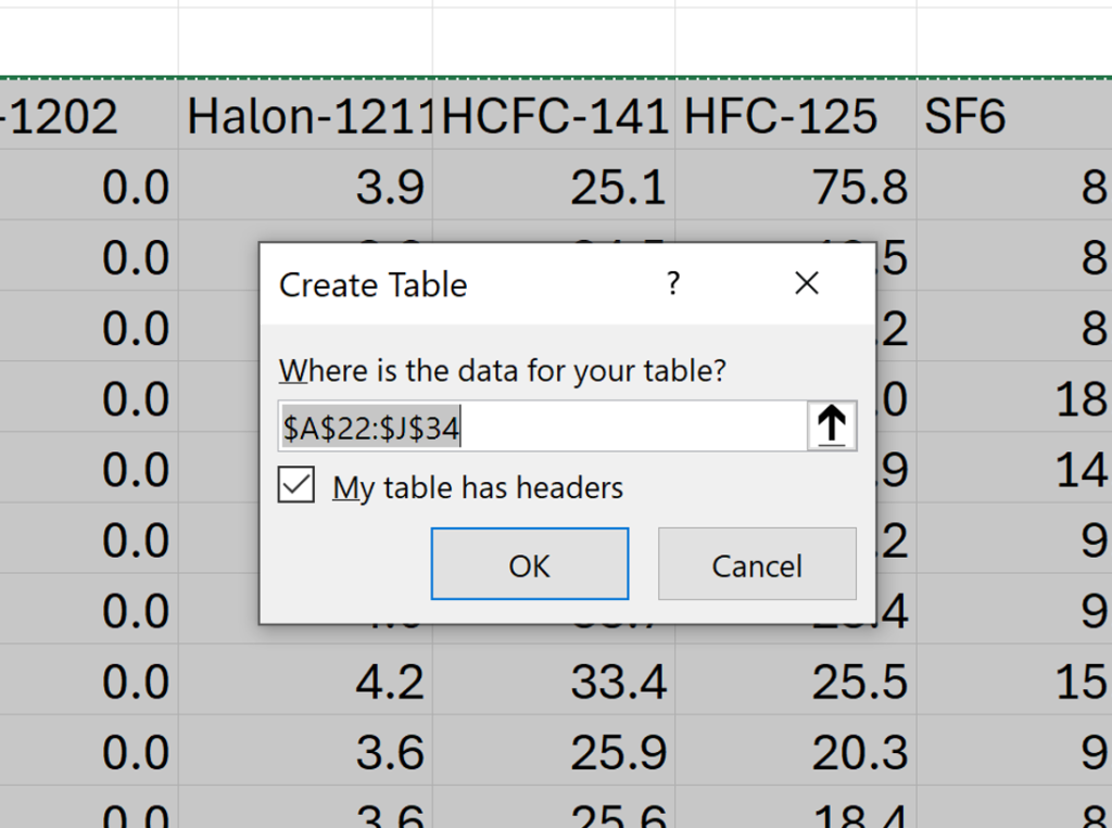
This will turn the range you have selected into an official excel table. Click OK.
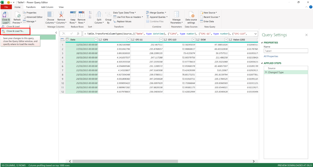
Then this will open your table in the Power Query Editor. Select Close & Load To…
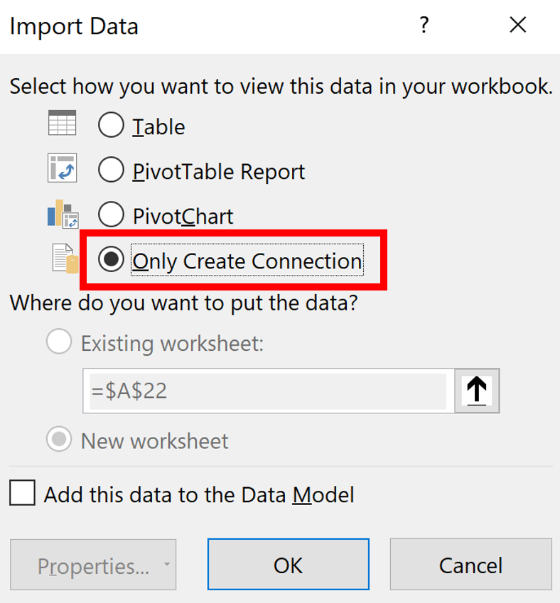
Next, select Only Create Connection and click OK. This will save your table as a Query.
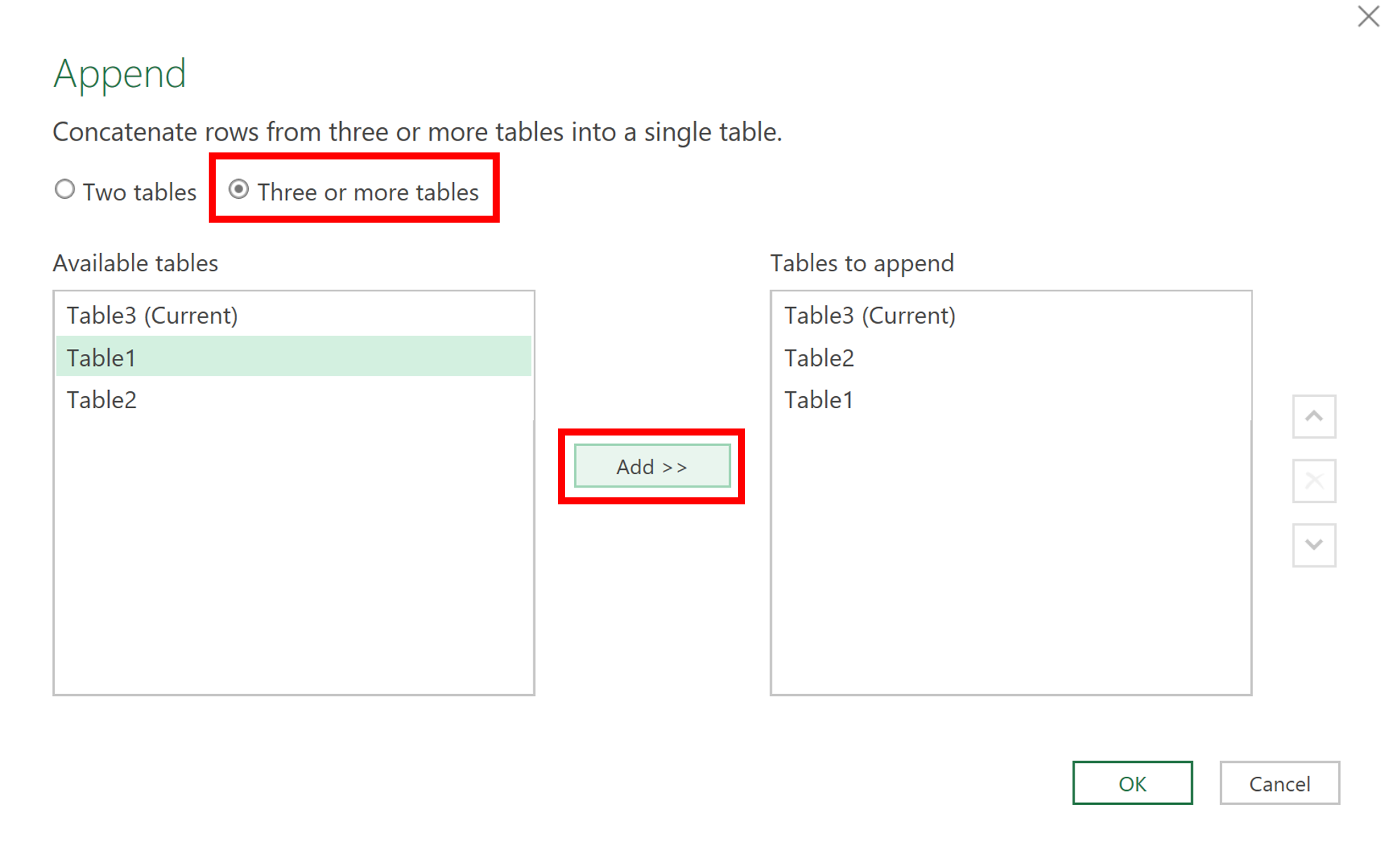
Do the same thing for all of your other tables. When you reach the first table, instead of closing it, click on Append Queries. This will allow you to add other queries to the bottom of your current query.
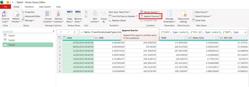
Select Three or more tables and Add your other tables and then click OK.

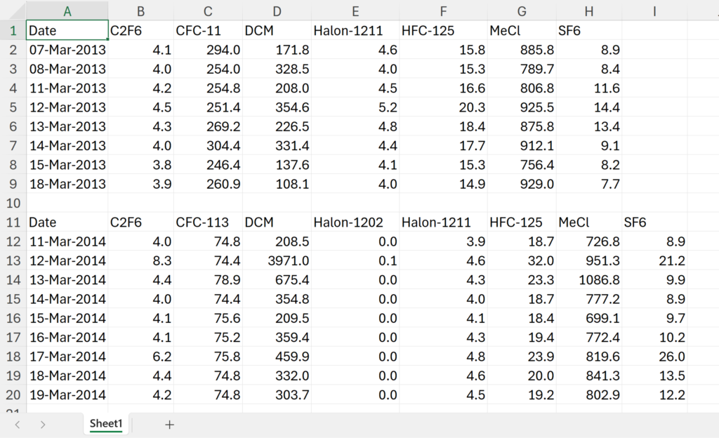
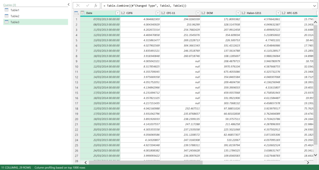
Now, the tables have been combined together, one on top of the other. Power Query automatically lines up the columns based on the column headings, and if a table does not have that column it fills the cells with null values.
Finally, go to Close & Load
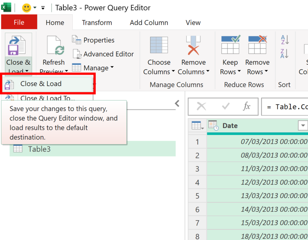
And this closed the Power Query Editor and loads your query as a table in a new worksheet.